Guide to Pitch Plots
Abhishek A. Mishra
2023-08-18
Source:vignettes/Guide_to_Pitch_Plots.Rmd
Guide_to_Pitch_Plots.RmdThis is the guide for using Pitch Plots in ggshakeR.
These plots aim to plot events on a pitch hence the name…Pitch Plots!
Currently, ggshakeR houses 7 Pitch Plots:
plot_pass()plot_heatmap()plot_sonar()plot_passflow()plot_shot()plot_convexhull()plot_voronoi()plot_passnet()
Let’s learn simple guides on how to use them!
Understat
plot_shot()
Characteristics:
- Only works with Understat data
- Has three types: hexbin, density, or point (default)
The easiest Pitch Plot function to use! To use this function, which only works with Understat data, we need the understatr package.
Once you have installed the package, put the package in your work session by writing:
library(understatr)We will use the understatr package to get the data for
plot_shot(). Browse through the understatr package to get
their data. As a sanity check, make sure the dataframe has columns with
these names:
-
X(not x) -
Y(not y) xGresultname
Here, I am going to get Mohammed Salah’s data. To learn more about how to get data, read Nandy’s excellent guide.
shot_data <- get_player_shots(player_id = 1250) # Salah's `player_id` on Understat is `1250`After that, simply write and execute the following code to get a beautiful shot map:
plot <- plot_shot(data, type = "density")

plot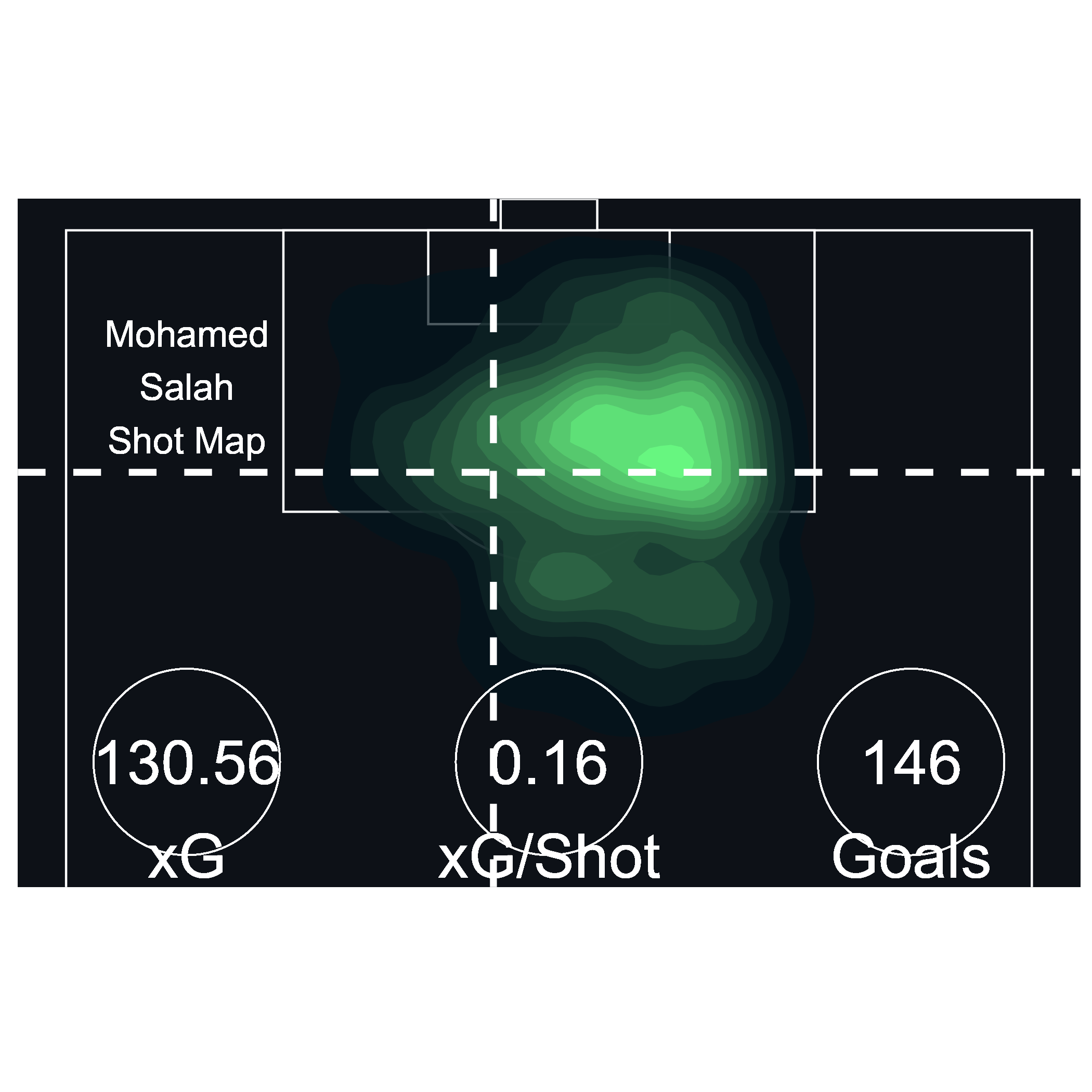
plot_shot() of Mohammed Salah
An additional feature is provided through a couple of other arguments within the function in the form of highlight_goals and average_location. Use them by toggling between TRUE and FALSE.
plot <- plot_shot(shot_data, highlight_goals = TRUE, average_location = FALSE)
plot
Note that, you can write “hexbin”, “density”, and “point” to get three different types of shot maps. However, the highlight_goals parameter only works for point shot maps. Try it out!
Opta & StatsBomb
plot_sonar(), plot_heatmap(),
plot_pass() & plot_passflow()
These three functions are quite similar in what they require.
-
plot_sonar()gives you a pass sonar -
plot_heatmap()gives you a heat map on the pitch -
plot_pass()gives you all the passes on the pitch -
plot_passflow()gives you a pass flow map on the pitch
Here are some key things to know:
plot_sonar(),plot_pass()andplot_passflow()expect passing dataAll three functions require the data to have at minimum four columns named: x, y, finalX, finalY
All three functions work on either Opta or Statsbomb data
-
All three functions need a minimum of 4 columns named:
-
x(indicates starting x location) -
y(indicates starting y location) -
finalX(indicates ending x location for passes) -
finalY(indicates ending y location for passes)
-
Let’s first get some data! You can either import you data or use Statsbomb’s open free dataset
In this example, I’ll be using StatsBomb’s Messi Data for La Liga 2014/15:
library(StatsBombR)

Comp <- FreeCompetitions() %>%
  filter(competition_id == 11 & season_name == "2014/2015")
Matches <- FreeMatches(Comp)
StatsBombData <- free_allevents(MatchesDF = Matches, Parallel = TRUE)
plotting_data  <- allclean(StatsBombData)
Before plotting, I am going to rename my columns:
plotting_data <- plotting_data %>%
  rename("x" = "location.x",
         "y" = "location.y",
         "finalX" = "pass.end_location.x",
         "finalY" = "pass.end_location.y")
Sweet, let’s plot!
plot_heatmap()
For the heat map, we simply select our columns and plot! Type options include bin, hex, density and jdp. Note that we don’t specify data_type since the default is set to “statsbomb”, so we can simply write this:
heat_data <- plotting_data %>%
  select(x, y)

heatPlot <- plot_heatmap(data = heat_data, type = "bin")

heatPlot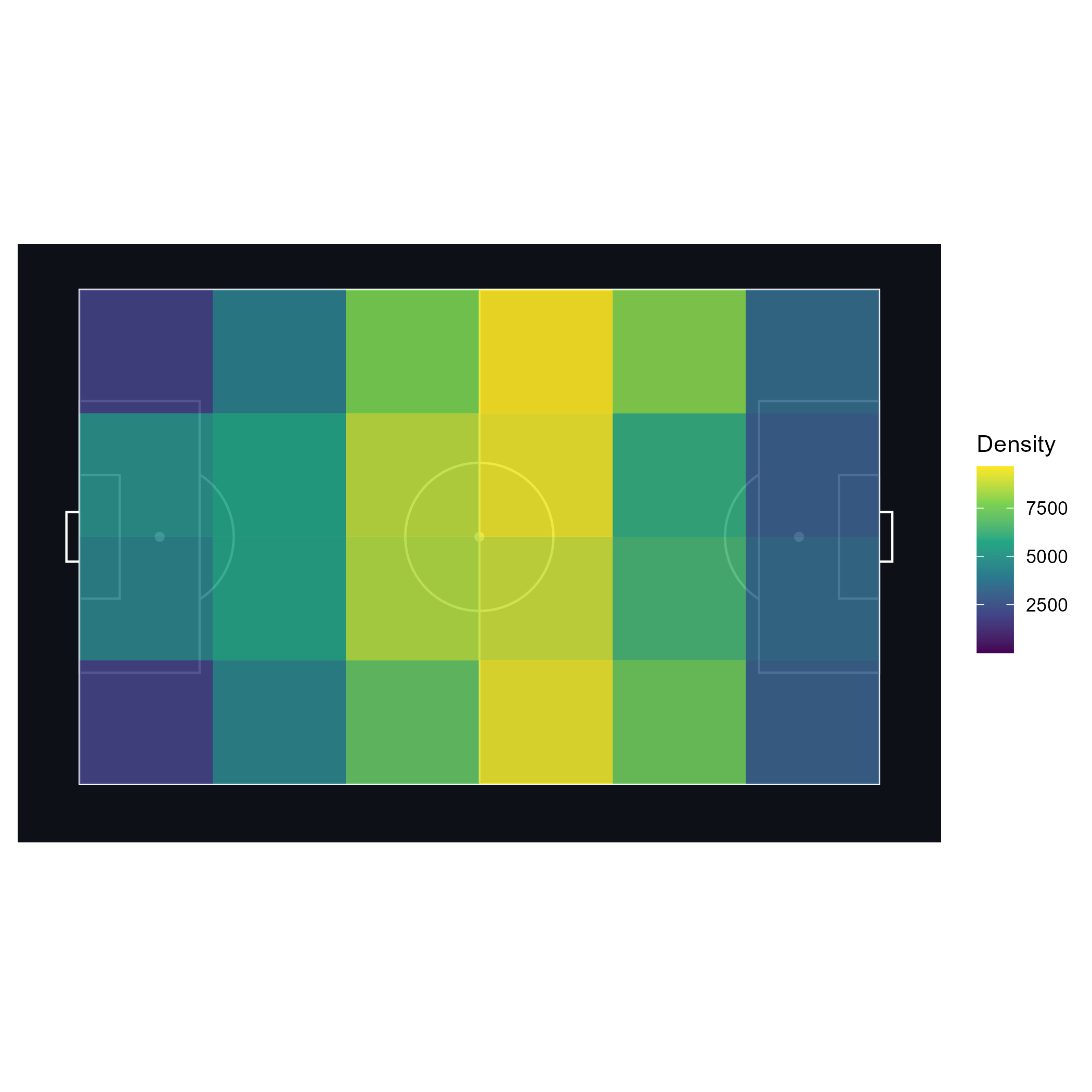
plot_heatmap() of all of La Liga’s events in 2014/15
plot_sonar()
For the pass sonar, we’re going to a bit more data cleaning. I don’t want everybody’s passing sonar - that’s redundant!
For our purposes, I want Jordi Alba’s passing sonar. First, let me get all passes from Jordi Alba:
plotting_data_alba  <- plotting_data %>%
  filter(type.name == "Pass" & team.name == "Barcelona" & player.name == "Jordi Alba Ramos")
Now I can construct a pass sonar! Default data_type is set to “statsbomb”, so here we can simply write:
sonarPlot <- plot_sonar(data = plotting_data_alba)

sonarPlot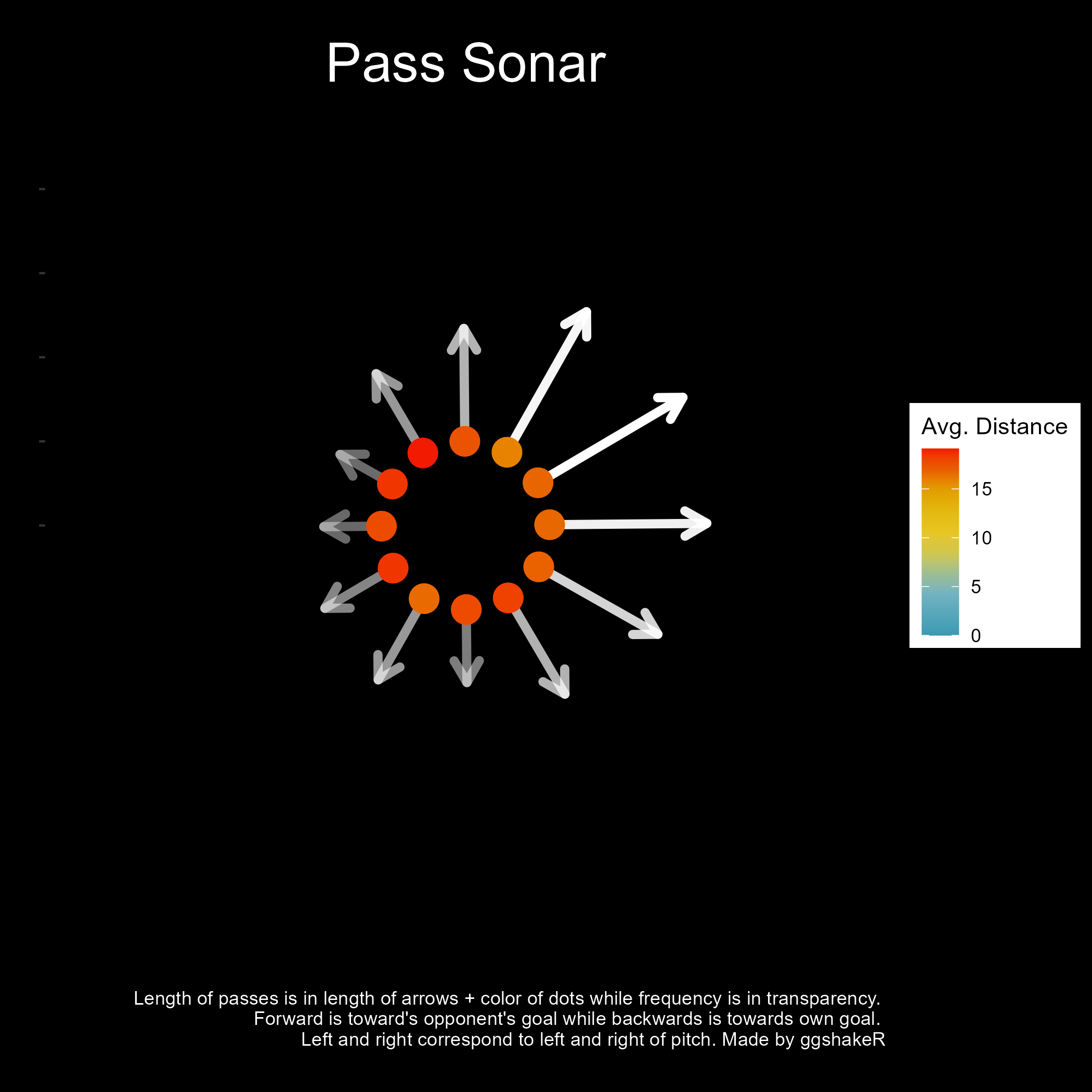
plot_sonar() of all of Jordi Alba’s passes from 2014/15
plot_pass()
We can create a pass map of all of Jordi Alba’s passes during a
particular match by using the plot_pass() function.
plotting_data_alba_single <- plotting_data_alba %>%
  filter(match_id == 70264)

passPlot <- plot_pass(data = plotting_data_alba_single,
                      progressive_pass = TRUE, type = "all")
passPlot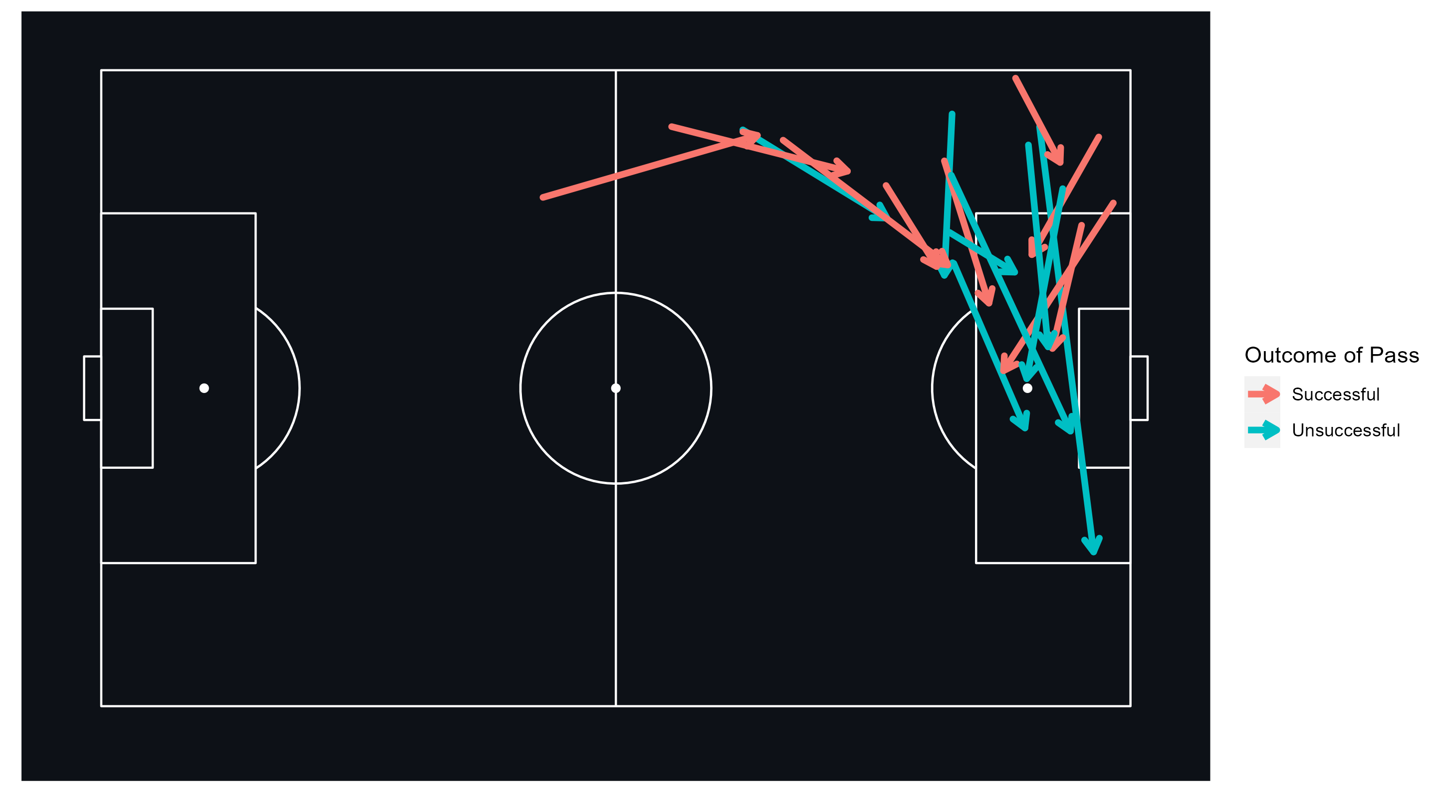
plot_pass() of all of Jordi Alba’s passes from a match in 2014/15
plot_passflow()
Since we already have Jordi Alba’s passes, we can just construct the pass flow like this:
passflowPlot <- plot_passflow(data = plotting_data_alba)

passflowPlot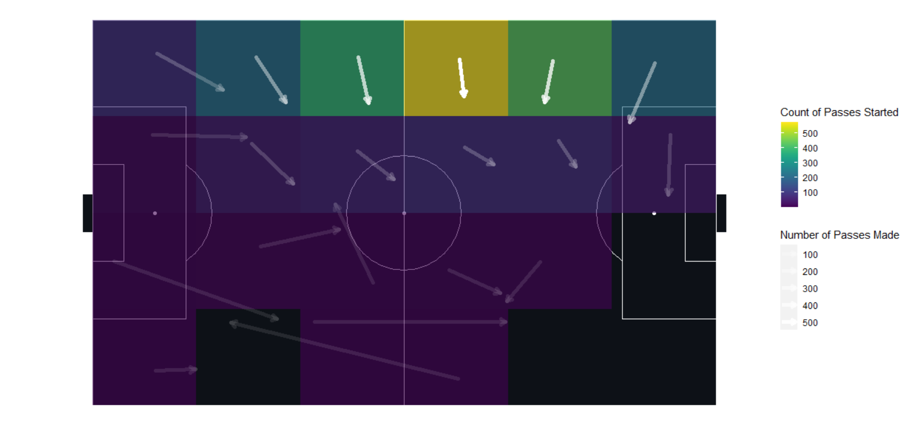
plot_passflow() of all of Jordi Alba’s passes from 2014/15
plot_convexhull()
This function allows the user to use event data to plot the convex hulls of multiple or a single player. It works on both Opta and StatsBomb data and requires the following columns:
xyfinalXfinalY-
playerId(Player name’s)
Let us plot using the data set we already have.
unique(plotting_data$match_id) # Find all match ID's from the data set

convexPlot <- plotting_data %>%
  filter(match_id == 266631,
         team.name == "Barcelona") %>%
  plot_convexhull()

convexPlot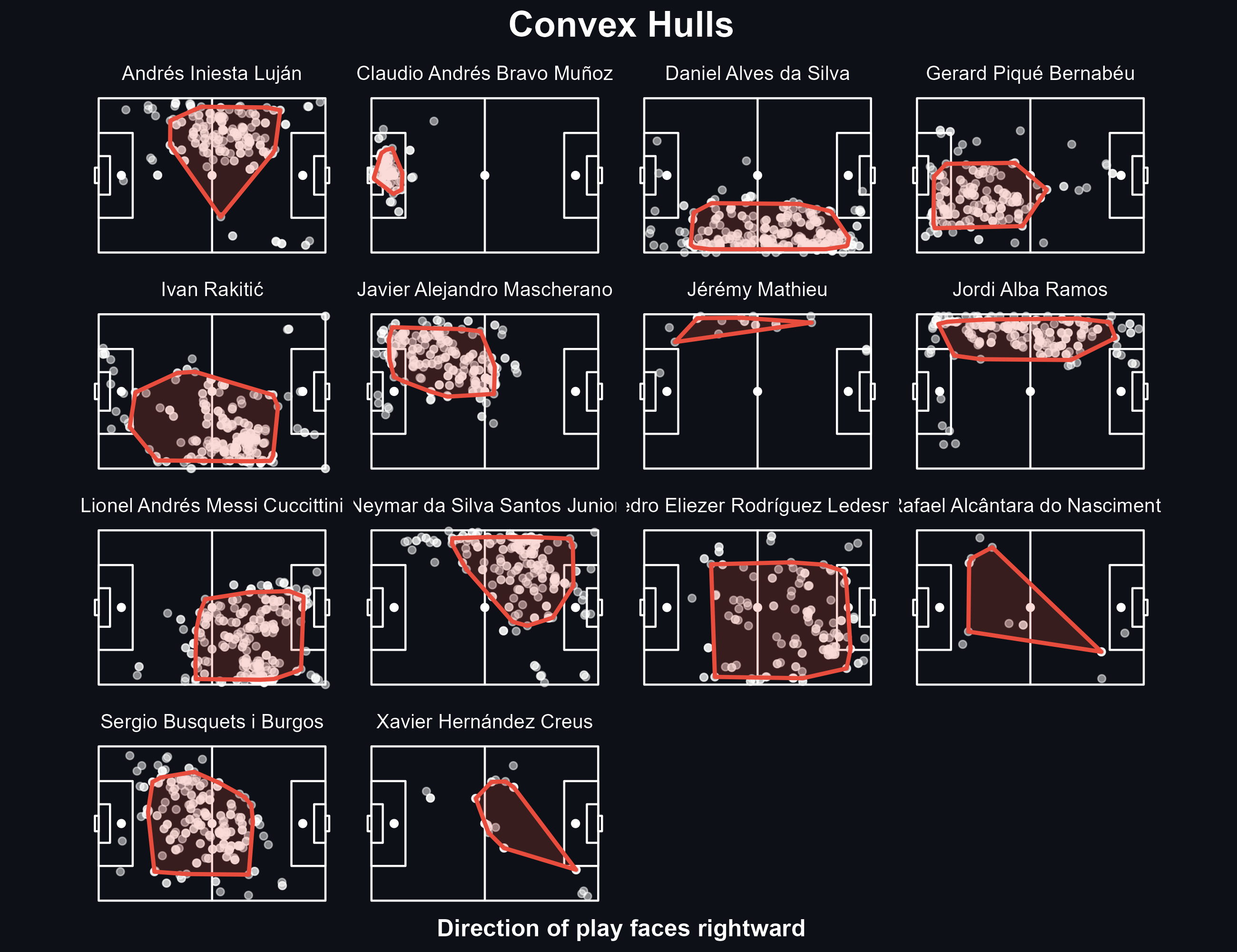
plot_convexhull() of FC Barcelona players from a match
Note that we do not need to pass any parameters to the function here as the data set has already been specified and the default data_type is set to “statsbomb”. If using Opta data, set the data_type as such. Manipulate the data set as per your needs and use-case. You can also plot a single player convex hull by filtering for the specific name in the pipe before applying the function. You can also alter the title and colors as you wish by using the relevant parameters.
Here is an example:
convexPlot <- plotting_data %>%
  filter(match_id == 266631,
         player.name == "Jordi Alba Ramos") %>%
  plot_convexhull(color = "#41ab5d", title = "Jordi Alba Convex Hull")

convexPlot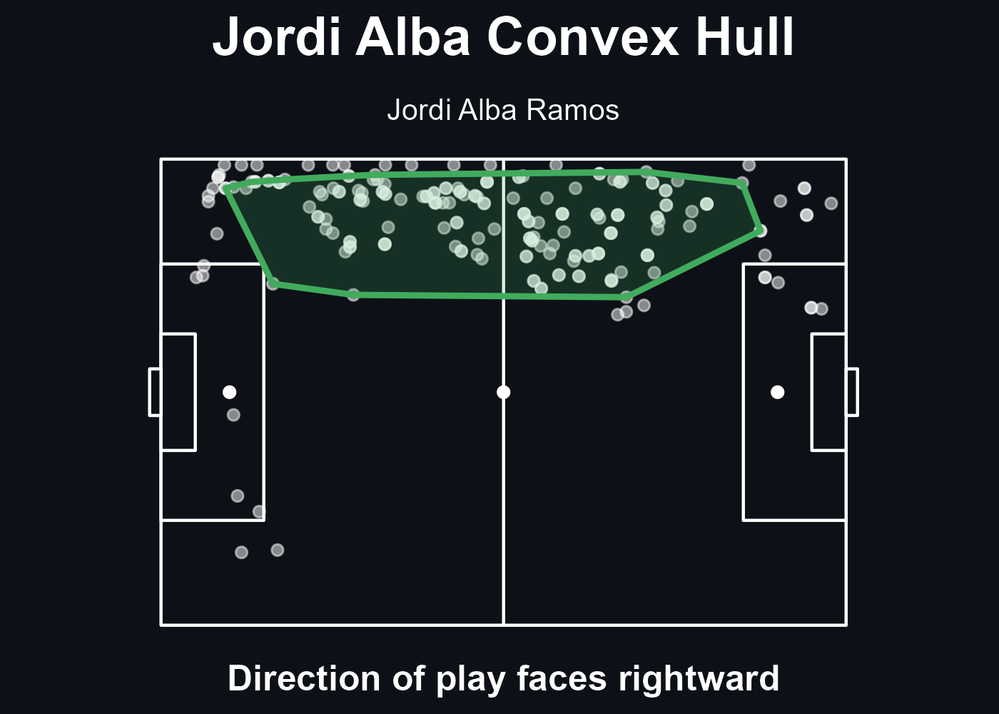
plot_convexhull() of all of Jordi Alba’s passes from a match
plot_voronoi()
This function allows the user to use event data to plot the voronoi plot of a set of points. It works on both Opta and StatsBomb data and requires the following columns:
xy
Let us plot using the data set we already have. First, we’ll get a summarized data set of players and their mean positions.
finalData <- plotting_data %>%
  filter(team.name == "Barcelona") %>%
  group_by(player.name) %>%
  summarise_at(vars(x, y, minute), list(name = mean), na.rm = TRUE) %>%
  na.omit() %>%
  rename("x" = "x_name") %>%
  rename("y" = "y_name")
After that, we can simply use the voronoi plot function:
plotVoronoi <- plot_voronoi(finalData)
plotVoronoi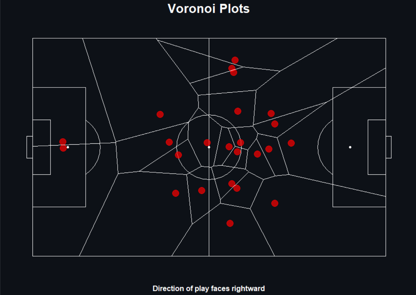
plot_voronoi() of FC Barcelona players and their mean positions
A note to remember, the voronoi plot works best when you have a summarized set of points.
For example, to see something like all of the start locations of a player’s passes, you would use convexhull() while to see how the team’s mean position for each player, you would use voronoi()
Note that we do not need to pass any parameters to the function here as the data set has already been specified and the default data_type is set to “statsbomb”. If using Opta data, set the data_type as such.
Manipulate the data set as per your needs and use-case. You can also fill the voronoi plots based on the values. You will need the fill value as another column. As usual, you can use piping to apply the function directly all in one line.
As an example, we will show EPV values calculated through
calculate_epv().
threatData <- calculate_epv(plotting_data)Once we have that, we will repeat the same code as before with a small change:
finalData <- threatData %>%
  filter(team.name == "Barcelona") %>%
  group_by(player.name) %>%
  filter(EPVStart != -1) %>% #Getting rid of -1 as that as how we identify null values
  #We get the mean and sum of these three columns
  summarise_at(vars(x, y, EPVStart), list(name = mean, sum), na.rm = TRUE) %>%
  na.omit() %>%
  rename("x" = "x_name") %>%
  rename("y" = "y_name") %>%
  rename("EPV_Start" =  "EPVStart_fn1") #Renaming the relevant columns

#Plot voronoi plot

plotVoronoi <- plot_voronoi(data = finalData,
                            fill = "EPV_Start",
                            title = "Barcelona Voronoi Diagram")
plotVoronoi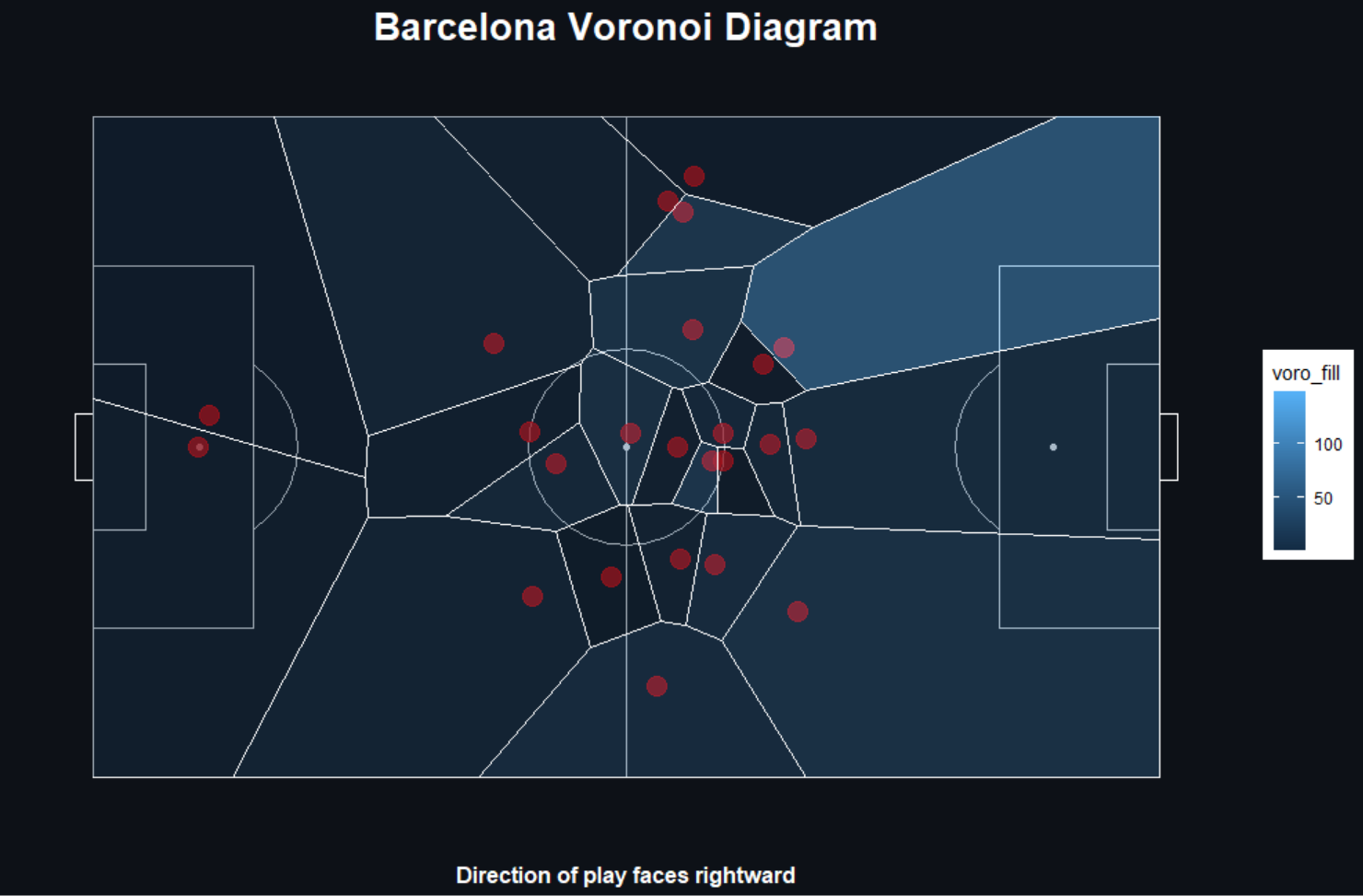
plot_voronoi() of FC Barcelona players and their mean positions with EPV
plot_passnet()
This function allows users to plot pass networks of a team in a particular match using event data from StatsBomb and Opta. Here we will be demonstrating how to use this function with both data types.
StatsBomb
Plotting a pass network with StatsBomb data is pretty simple. All you
need is a standard StatsBomb data set with the 4 coordinate columns
being renamed to x, y, finalX and
finalY, in line with what we have done for all other
functions so far. We select a specific match and then plot away!
unique(plotting_data$match_id) # Find all match ID's from the data set

passnetPlot <- plotting_data %>%
  filter(match_id == 266631) %>%
  plot_passnet(team_name = "Barcelona")

passnetPlot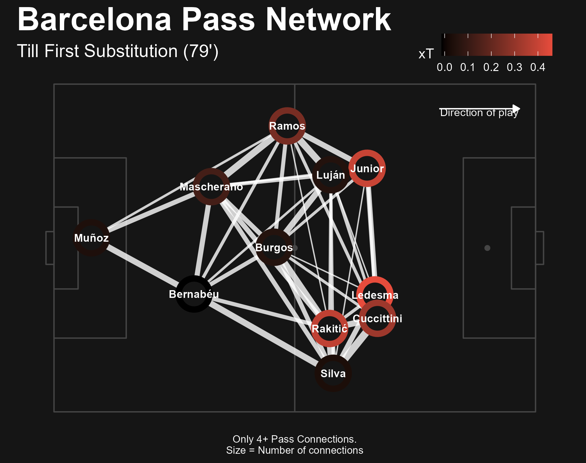
plot_passnet() of FC Barcelona in a match
team_name is the one parameter that needs to be used here, as the all other parameters have been set to their default. Work with different colors using the scale_color parameter, different stats using scale_stat and alter the subtitle with subtitle if you wish to do so!
Opta
Using plot_passnet() with Opta data is a bit more
complicated. But fear not! We will be guiding you through the entire
process so that you get the hang of it. Firstly you need an Opta data
set. We created a data set to perfectly mimic an Opta data set and it is
available within the package for your use. Call it by running:
optadata <- ggshakeR::SampleEventDataNow that you have your data set, let us see which columns we require for our function:
xyfinalXfinalYminute-
playerId(Player name’s) -
teamId(Team name’s) -
outcome(Outcome of the pass) -
type(Type of event)
Note that the playerId and teamId columns need to contain player and team names. The data set in our hands only contains their relevant Id’s. Let us fix that and transform the data set into one that will be accepted by our function.
optadata <- optadata %>%
  mutate(teamId = case_when(teamId == 2151 ~ "Team 1",
                            teamId == 3070 ~ "Team 2")) %>%
  mutate(playerId = case_when(playerId == "1" ~ "Cameron",
                              playerId == "2" ~ "Sahaj",
                              playerId == "3" ~ "Trevor",
                              playerId == "4" ~ "Jolene",
                              playerId == "5" ~ "David",
                              playerId == "6" ~ "Marcus",
                              playerId == "7" ~ "Ryo",
                              playerId == "8" ~ "Anthony",
                              playerId == "9" ~ "Aabid",
                              playerId == "10" ~ "Kylian",
                              playerId == "11" ~ "Harry",
                              playerId == "12" ~ "Victor",
                              playerId == "13" ~ "Jesse",
                              playerId == "14" ~ "Borges",
                              playerId == "15" ~ "Miguel",
                              playerId == "16" ~ "Alex",
                              playerId == "17" ~ "Abdul",
                              playerId == "18" ~ "Eric",
                              playerId == "19" ~ "Marten",
                              playerId == "20" ~ "Robert",
                              playerId == "21" ~ "Lionel",
                              playerId == "22" ~ "Dean",
                              playerId == "23" ~ "Aaron",
                              playerId == "24" ~ "Benjamin",
                              playerId == "25" ~ "Diego",
                              playerId == "26" ~ "Abhishek",
                              playerId == "27" ~ "Samuel",
                              playerId == "28" ~ "Edward",
                              playerId == "29" ~ "Malik",
                              playerId == "30" ~ "Albert",
                              playerId == "31" ~ "Paul",
                              playerId == "32" ~ "Smith",
                              playerId == "33" ~ "Seth",
                              playerId == "34" ~ "Mohammed",
                              playerId == "35" ~ "Eder",
                              playerId == "36" ~ "Adam",
                              playerId == "37" ~ "Harsh",
                              playerId == "38" ~ "Jorge",
                              playerId == "39" ~ "Zak",
                              playerId == "40" ~ "Brandon"))
Here we have used the case_when() function to link the
player and team Id’s to the relevant names. There is still some work
left to do.
optadata <- optadata %>%
  rename(finalX = endX,
         finalY = endY)
We have cleaned up our data set. It is now ready to be used in the function.
It is important to note that these steps might not be necessary for all data sets. This is only to make sure that we are following the correct format for the function. A data set with these exact column names and column type specifications will work within the function without any errors.
Let us now plot.
passnetPlot <- plot_passnet(data = optadata, data_type = "opta",
                            team_name = "Team 1", scale_stat = "EPV",
                            scale_color = "#fec44f")

passnetPlot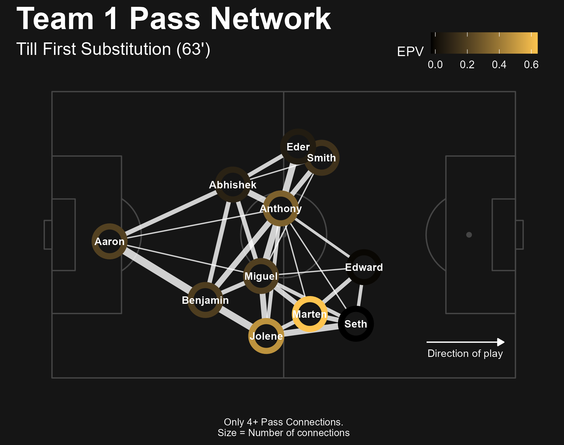
plot_passnet() using opta data
Contributors
There are a few people to credit with helping in the creation of the pitch plot functions.
The design for plot_sonar() is inspired by the pass
compass plot designed by e. Part of the sonar
production code is also credited to Eliot McKinley.
Credit to Joe
Gallagher and his excellent package soccermatics for the
code used for data wrangling in the plot_passnet()
function.