Guide to Expected Threat
Abhishek A. Mishra
2023-08-18
Source:vignettes/Guide_to_Exp_Threat.Rmd
Guide_to_Exp_Threat.RmdWelcome to the Expected Threat Guide for ggshakeR!
First things first, we are only able to do this because of the amazing work by Karun Singh. Read his excellent xT blog post that goes into in-depth explanation of the need and use of the metric.
Karun Singh’s xT grid is what ggshakeR uses. Every time you load in the package, ggshakeR will load in a dataframe called xTGrid. xTGrid houses all the xT data that Karun Singh made public and now it is available for you in a line of code!
Simply write:
This dataframe is there for you to use and play with. The columns correspond to pitch divisions from your own goal (X0) to the opponent’s goal (X11). The grid is symmetrical in half and as such, there is no “top”/“bottom” of the pitch.
However, what if you want to use xT? Calculate it?
ggshakeR offers you the calculate_threat() function that
calculates xT for the data that is passed in!
Here are some characteristics:
- Needs 4 columns named as
x,y,finalX,finalY.
Here’s the cool thing about the calculate_threat()
function: It calculates the xT of the start of a pass/carry and
the xT of the end of the pass/carry.
Why is this important? Well, let’s take a take-on. That only has a
starting x ,y . In the dataframe, the columns
of finalX and finalY have NAs in
them. The calculate_threat() will give you the xT for both
the starting and ending locations allowing you to give a value to
single-event values - basically, it gives you the most freedom and
information regarding xT.
Let’s see how we can use it!
Using the calculate_threat() function
First, let’s get some data! You can either import you data or use Statsbomb’s open free dataset
In this example, I’ll be using StatsBomb’s Messi Data for La Liga 2014/15:
library(StatsBombR)

Comp <- FreeCompetitions() %>%
  filter(competition_id == 11 & season_name == "2014/2015")
Matches <- FreeMatches(Comp)
StatsBombData <- free_allevents(MatchesDF = Matches, Parallel = TRUE)
StatsBombData <- allclean(StatsBombData)

plottingData <- StatsBombData
Before plotting, I am going to rename my columns:
plottingData <- plottingData %>%
  rename("x" = "location.x",
         "y" = "location.y",
         "finalX" = "pass.end_location.x",
         "finalY" = "pass.end_location.y")
For calculate_threat(), always write the type
that the data is: opta or statsbomb. After that, we simply
get:
## NOTE: from version 0.2.0 ALL function arguments are now in snake_case
## 'dataType' is now 'data_type', etc.
xTData <- calculate_threat(data = plottingData, type = "statsbomb")
If we inspect xTData, we see these two new columns at
the very end:
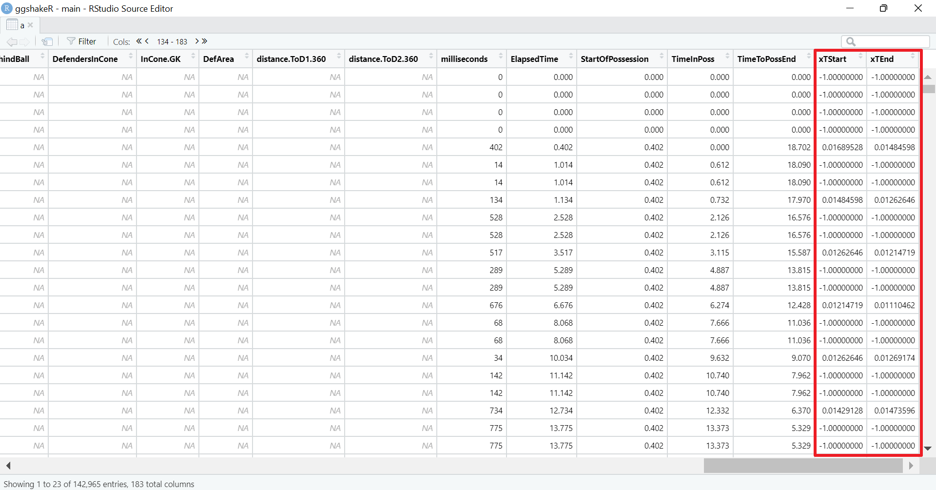
calculate_threat() producing xTStart and xTEnd
As you’ll see, calculate_threat() will put a -1 in areas
where there was a value that was not right for calculation. To calculate
the difference in xT, simply write:
xTData <- xTData %>%
  mutate(xT = xTEnd - xTStart)
This will give you the difference in xT and this value can be used
for passes, carries - anything that has a start and an end location. Use
xTStart/xTEnd for single-occuring events such
as take-ons, tackles, if you so wish.