Guide to Expected Possession Value

Abhishek A. Mishra

2023-08-18

Welcome to the Expected Possession Value Guide for ggshakeR!

EPV - short for Expected Possession Value - is one of the most popular and informative metrics out there! Measuring the probability that an action leads to a goal, EPV allows you to objectively calculate passes, carries, and other events.

EPV was developed by Javier Fernández, Luke Bornn & Daniel Cervone.

There are various iterations of EPV that exist out there. OptaPro has their own PV while StatsBomb has something similar with their OBV.

The only publicly available data regarding EPV comes from Laurie Shaw who made an EPV grid public with his work with Friends of Tracking

Laurie Shaw’s EPV grid is what ggshakeR uses.

Every time you load in the package, ggshakeR will load in a dataframe called EPVGrid. EPVGrid houses all the EPV data that Laurie Shaw made public and now it is available for you in a line of code!

Simply write:

library(ggshakeR)

head(EPVGrid)

This dataframe is there for you to use and play with. The columns correspond to pitch divisions from your own goal (V1) to the opponent’s goal (V50). The grid is symmetrical in half and as such, there is no “top”/“bottom” of the pitch.

However, what if you want to use EPV? Calculate it?

ggshakeR offers you the calculate_epv() function that calculates EPV for the data that is passed in!

Here are some characteristics:

• Needs 4 columns named as x, y, finalX, finalY.

Here’s the cool thing about the calculate_epv() function: It calculates the xT of the start of a pass/carry and the xT of the end of the pass/carry.

Why is this important? Well, let’s take a take-on. That only has a starting x ,y . In the dataframe, the columns of finalX and finalY have NAs in them. The calculate_epv() will give you the EPV for both the starting and ending locations allowing you to give a value to single-event values.

This means, you can use this function beyond passes and carries and be able to calculate EPV for clearances, tackles, take-ons, etc! In addition, by separating out the EPV values for the start and end, you can apply more advanced analytics to the passes.

Let’s see how we can use it!

Using the calculate_epv() function

First, let’s get some data! You can either import you data or use Statsbomb’s open free dataset

In this example, I’ll be using StatsBomb’s Messi Data for La Liga 2014/15:

library(StatsBombR)

Comp <- FreeCompetitions() %>%
  filter(competition_id == 11 & season_name == "2014/2015")
Matches <- FreeMatches(Comp)
StatsBombData <- free_allevents(MatchesDF = Matches, Parallel = TRUE)
StatsBombData <- allclean(StatsBombData)

plottingData <- StatsBombData

Before plotting, I am going to rename my columns:

plottingData <- plottingData %>%
  rename("x" = "location.x",
         "y" = "location.y",
         "finalX" = "pass.end_location.x",
         "finalY" = "pass.end_location.y")

For calculate_epv(), always write the type that the data is: opta or statsbomb. After that, we simply get:

EPVData <- calculate_epv(plottingData, type = "statsbomb")

If we inspect EPVData, we see these two new columns at the very end:

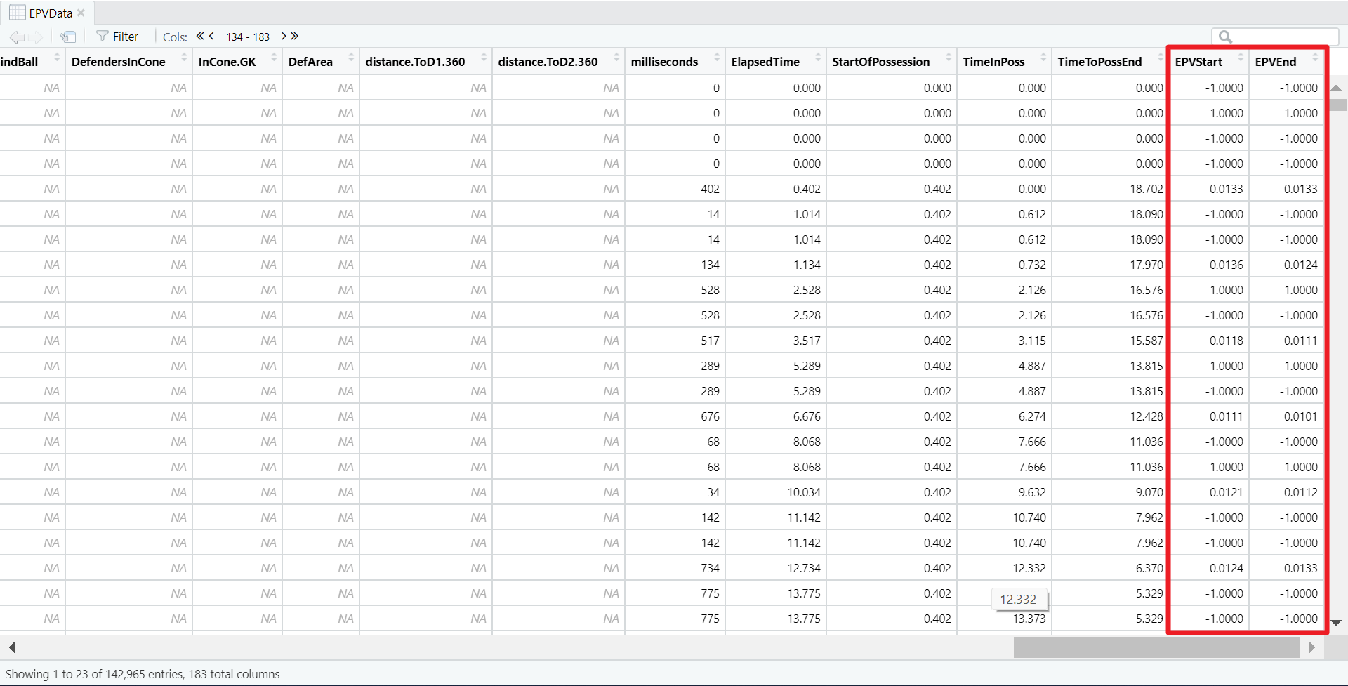
calculate_epv() producing EPVStart and EPVEnd

As you’ll see, calculate_epv() will put a -1 in areas where there was a value that was not right for calculation. To calculate the difference in EPV, simply write:

EPVData <- EPVData %>%
  mutate(EPV = EPVEnd - EPVStart)

This will give you the difference in EPV and this value can be used for passes, carries - anything that has a start and an end location. Use EPVStart/EPVEnd for single-occuring events such as take-ons, tackles, if you so wish.